How to Find, Highlight & Remove Duplicates in Google Sheets [Step-by-Step]

Duplicate information is the bane of spreadsheet options, particularly at scale. Given the quantity and number of information now entered by groups, it’s attainable that duplicate information in instruments like Google Sheets could also be related and essential, or it may very well be a irritating distraction from the first objective of spreadsheet efforts.

The potential downside raises query: How do you spotlight duplicates in Google Sheets?

I’ve received you coated with a step-by-step take a look at how you can spotlight duplicates in Google Sheets and discover duplicates in Google Sheets, full with pictures to make sure you’re heading in the right direction on the subject of de-duplicating your information.

Desk of Contents

The right way to Discover Duplicates in Google Sheets

Google Sheets is a free, cloud-based different to proprietary spreadsheet applications and — no shock, because it’s Google we’re coping with — provides a bunch of nice options to assist streamline information entry, formatting, and calculations.

There are two methods to take away duplicates in Google Sheets: conditional formatting and the UNIQUE operate. I’ll go over each under, however, earlier than you begin following alongside, I’ve two issues to notice: 

1. You may run a number of conditional formatting guidelines at a time, so that you don’t must delete any to run your conditional formatting rule to delete duplicates. 
2. You gained’t get an correct duplicate rely when you have any further characters or areas in your information, so you could ensure that your set is clear. Even an unintentional further area will rely it as a separate information level.

Let’s dive into how one can spotlight and take away duplicates in Google Sheets. 

Highlighting Duplicate Knowledge in Google Sheets

Google Sheets has all of the acquainted features: File, Edit, View, Format, Knowledge, Instruments, and many others., and makes it straightforward to rapidly enter your information, add formulas for calculations, and uncover key relationships. 

Whereas different spreadsheet instruments, such as Excel, have built-in conditional formatting instruments to pinpoint duplicate information in your sheet, Google’s answer requires a little bit extra guide effort. 

So how do you routinely spotlight duplicates in Google Sheets? Whereas there’s no built-in software for this objective, you may leverage some built-in features to focus on duplicate information.

Step-by-Step: The right way to Spotlight Duplicates in Google Sheets (With Photos)

Right here’s a step-by-step information to highlighting duplicates in Google Sheets:

Step 1: Open your spreadsheet.

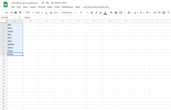
Step 2: Spotlight the info you need to verify.

Step 3: Below “Format”, choose “Conditional Formatting.”

Step 4: Choose “Customized formulation is.”

Step 5: Enter the customized duplicate checking formulation.

Step 6: Click on “Carried out” to see the outcomes.

Step 1: Open your spreadsheet.

First, head to Google Sheets and open the spreadsheet you need to verify for duplicate information.

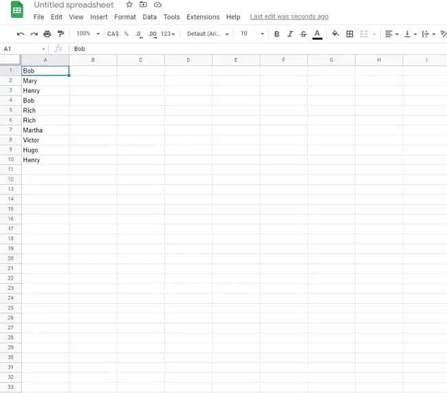
Step 2: Spotlight the info you need to verify.

Subsequent, drag your cursor over the info you need to verify to focus on it.

Step 3: Below “Format”, choose “Conditional Formatting.”

Now, head to “Format” within the high menu row and choose “Conditional Formatting.” It’s best to then see a popup window titled “Conditional format guidelines.” 

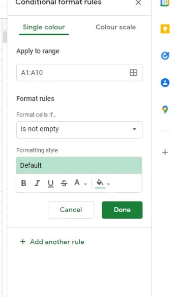
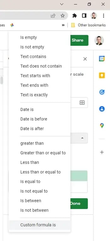
Step 4: Choose “Customized formulation is.”

Subsequent, you could create a customized formulation. Click on the down arrow beneath “Format cells if,” and choose “Customized formulation is” from the dropdown menu. It’s the final possibility to select from, so you may scroll proper to the tip.

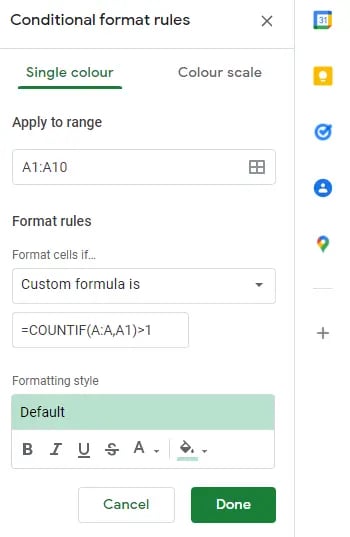
Step 5: Enter the customized duplicate checking formulation.

To seek for duplicate information, we have to enter the customized duplicate checking formulation, which for our column of information (A) seems like this:

=COUNTIF(A:A,A1)>1

The formulation searches for any textual content string that seems greater than as soon as in an information set. The default spotlight shade is inexperienced, however you may change it by clicking on the paint can icon within the “Formatting fashion” menu. 

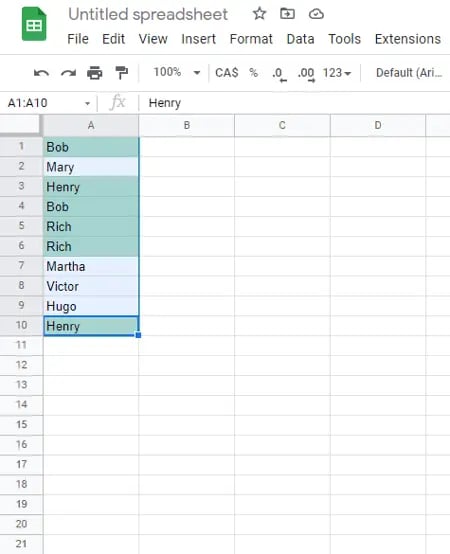
Step 6: Click on “Carried out” to see the outcomes.

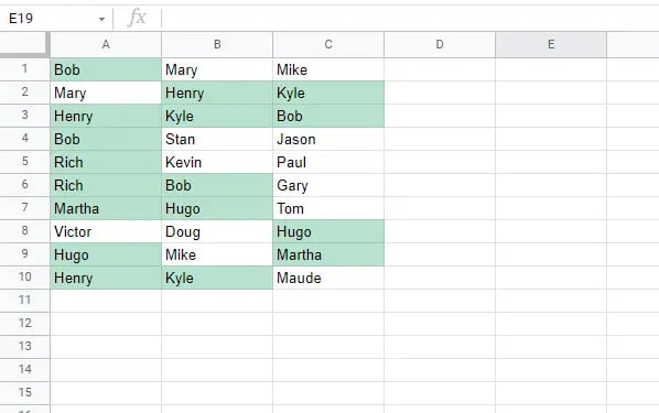
And voilà — we’ve highlighted the duplicate information in Google Sheets.

The right way to Spotlight Duplicates in A number of Rows and Columns

You may also spotlight duplicates in a number of rows and columns when you have a bigger information set. The method begins the identical as above, however you enter an expanded information vary within the Conditional format guidelines menu to account for all of the cells you need to examine. 

I’ll use the identical instance above as a place to begin, however I’ll add just a few extra names so we use a formulation to go looking throughout three columns: A, B, and C, and in addition throughout rows 1-10.

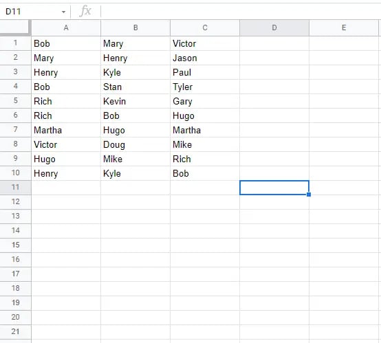
To begin, repeat steps two – 4 from above, however enter the next equation throughout step 5: 

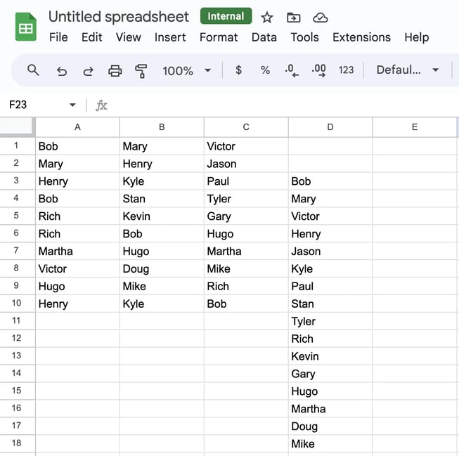
=COUNTIF($A$2:G,Oblique(Tackle(Row(),Column(),)))>1

It will spotlight all duplicates throughout all three columns and all ten rows, making it straightforward to identify information doppelgangers:

Discover and Spotlight Duplicates in Google Sheets With the Distinctive Perform

One other strategy to discover duplicates in Sheets is to make use of the UNIQUE operate, which seems for the distinctive values in your designated vary and produces a duplicate-free listing. Right here’s the formulation: 

=UNIQUE(RANGE)

Notice: This formulation can solely establish duplicates in a single column. 

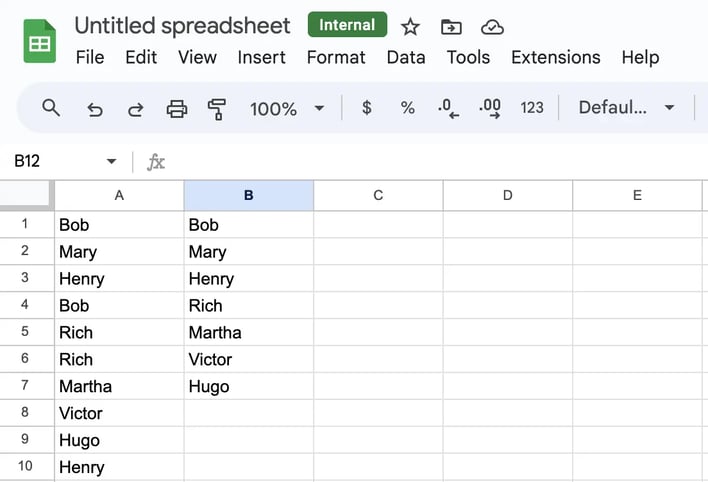
There’s just one step to this technique, which is coming into your formulation into an empty cell. Persevering with with the identical information set from above, I entered =UNIQUE(A1:A10). The picture under is my duplicate-free listing (on the left).

To make use of the UNIQUE operate to search out duplicates in a number of columns and rows, use this formulation: 

 =UNIQUE(TOCOL(RANGE))

A disadvantage to utilizing the UNIQUE operate to search out duplicates in Google Sheets is that it spits out a separate duplicate-free listing as an alternative of highlighting and deleting them. It creates an added step because you’ll should manually take away duplicates together with your new listing as a reference, so I like to recommend this technique for these with a smaller information set who don’t thoughts just a few guide updates. 

Alternatively, this technique is a superb possibility for producing a cleaned listing to start out contemporary.

The right way to Take away Duplicates in Google Sheets

Along with highlighting duplicates, you may as well use Google Sheets to delete duplicates with the Knowledge Cleanup function. Beneath, I’ll present you the way.

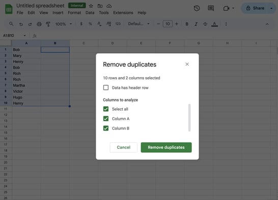
Step 1: Choose any cell.

Step 2: Navigate to the header toolback, choose “Knowledge,” then “Knowledge cleanup,” then “Take away duplicates.”

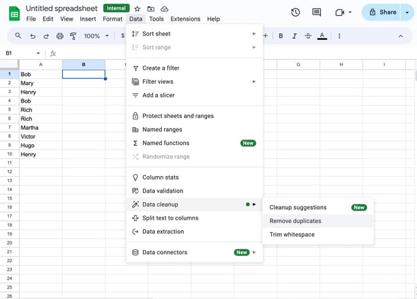
Step 3: Within the popup window, choose the columns you need to delete duplicate information from, then choose “Take away duplicates.

Notice: When you’ve got a sheet header, ensure that to pick out “Knowledge has a header row” so it’s not included within the duplicate search. 

All duplicates are actually gone!

Dealing With Duplicates in Duplicates in Google Sheets

Are you able to spotlight duplicates in Google Sheets? Completely. Whereas the method takes extra effort than another spreadsheet options, it’s straightforward to duplicate when you’ve executed it a couple of times, and when you’re comfy with the method you may scale as much as discover duplicates throughout rows, columns, and even a lot bigger information units.